

Source: Hu, Edward, et al, LoRA: Low-Rank Adaptation of Large Language Models, 2021
Fine-Tuning Smarter, Not Harder:
Modern models are huge. Updating every parameter of a transformer for each new task is wasteful when most of what the model knows is already useful. LoRA (Low-Rank Adaptation) offers a neat compromise: keep the foundation fixed and learn a tiny, targeted update that steers the model to your task with almost no extra memory.
Instead of updating the full pretrained weight matrix $\mathbf{W} \in \mathbb{R}^{d \times d}$, LoRA introduces two small low-rank matrices $\mathbf{A}$ and $\mathbf{B}$ that capture task-specific adaptations. The input $x$ is first projected through the frozen pretrained weights $\mathbf{W}$, and a learned low-rank update $\mathbf{BA}x$ is added to produce the output $h$. Matrix $\mathbf{A}$ is initialized with small random values (e.g., $\mathcal{N}(0, \sigma^2)$), while $\mathbf{B}$ is typically initialized to zero so that the network initially behaves like the pretrained model. During fine-tuning, only $\mathbf{A}$ and $\mathbf{B}$ are updated, keeping $\mathbf{W}$ fixed, making LoRA an efficient, low-memory adaptation method.
The General Idea
For a pretrained weight $W_0 \in \mathbb{R}^{d\times k}$, full fine-tuning learns a dense update $\Delta W$. LoRA constrains that update to a low-rank form:
During training the effective weight is:
with scale $\alpha$. Only $A$ and $B$ receive gradients,
so the frozen backbone stays intact and the update lives on the low-rank manifold $\mathcal{M}_r={BA}$.
Most task-specific adjustments lie in a small number of directions. If we learn just those, we get most of the benefit for a fraction of the cost.
A quick example
Suppose a layer has $W_0\in\mathbb{R}^{1024\times1024}$ ($~1.05M$ params). With rank $r=8$, LoRA learns
$A\in\mathbb{R}^{8\times1024}$ and $B\in\mathbb{R}^{1024\times8}$: $~16k$ parameters total, well under $2\%$ of the full layer, yet the product $BA$ can express the “direction” of the useful update. After training, $BA$ can be merged into $W_0$ and inference cost is unchanged.
What we trained (and why)
In the accompanying notebook (coming soon), we fine-tune DistilBERT on IMDb sentiment (binary). We compare:
- Frozen (linear probe) : freeze the encoder, train only the classifier head
- Full fine-tune : update all weights
- LoRA : adapters on attention $q,v$ projections ($r=8, \alpha=16$)
We train first, then visualize results:
| Model | Accuracy | Trainable Params |
| Frozen (linear probe) | 0.742 | 592,130 |
| Full Fine-Tune | 0.834 | 66,955,010 |
| LoRA (r=8) | 0.799 | 739,586 |

Source: AIML.com Research
In this run, LoRA sits within $~3$ to $4$ points of full fine-tuning while training $~90×$ less parameters. The linear probe is a fast baseline that lags, as expected.
Beyond accuracy: what the curves say
We plot all three ROC curves together and all three PR curves together.

Source: AIML.com Research

Source: AIML.com Research
Both views tell a consistent story: LoRA tracks full FT closely across thresholds, while the linear probe underperforms at higher recall. Full FT reduces false negatives the most. This is how often the model misses positive cases (e.g., predicting “negative” for a positive true outcome). LoRA lands between full FT and the linear probe, with balanced errors.
Efficiency matters
Parameter count is strategy. A single base model can serve many tasks by swapping tiny LoRA weights; storage and deployment become modular. In other words, you can fine-tune models on consumer hardware (as opposed to large-scale academic or research group hardware) without retraining the entire network. This technique allows you to experiment with several downstream tasks, depending on your needs.

Source: AIML.com Research
We also experimented with LoRA rank (r) over $\{2,4,8,16, 100\}$. Accuracy improves and then saturates quickly, showing that small ranks capture most of the gain. I included rank $100$ to showcase how the plateau is real and there is no need to go that high, at least for the current model and dataset.

Source: AIML.com Research
Rule of thumb. Pick the largest $r$ that fits memory; scale $\alpha$ roughly with $r$ (e.g., $\alpha\approx2r$) so the effective update $(\alpha/r)BA$ has stable magnitude.
In this example, accuracy at rank 2 was around 0.76, improved to 0.80 at rank 4, and saturated thereafter, even at rank 100, improving slightly. Mathematically, this happens because most of the update energy lies in a few singular directions. Once $r$ covers the top singular components of the true update $\Delta W$, additional rank adds redundant capacity with diminishing returns.
Here is a simple code snippet that explains the above. This small configuration is often enough to replicate most of the benefits of full fine-tuning while using $<2\%$ of the trainable parameters.
from peft import LoraConfig, get_peft_model

config = LoraConfig(
    r=8,              # Rank of the low-rank matrices
    lora_alpha=16,    # Scaling factor (≈ 2r is a good starting point)
    target_modules=["q_proj", "v_proj"],  # Layers to adapt
    lora_dropout=0.05 # Regularization
)

model = get_peft_model(base_model, config)Why LoRA works
LoRA succeeds because of both mathematical structure and practical advantages:
- Low-rank redundancy. Pretrained features are highly correlated; useful task updates occupy a low-dimensional subspace
- Regularization. Constraining updates to $\mathcal{M}_r$ prevents overfitting and keeps optimization stable
- Modularity. Adapters are small files you can mix and match per task or domain
- Operational wins. Smaller checkpoints, lower memory, and quicker iterations, especially valuable on laptops and edge devices
When (not) to reach for LoRA
Choose LoRA when you have limited compute or need many task-specific variants. Use full FT when the domain shift is severe and every layer likely needs substantial change. As a fast baseline, a linear probe is still handy to establish how much the frozen backbone already knows.
Closing
LoRA delivers most of the benefit of full fine-tuning at a fraction of the cost by learning only the directions that matter. For practitioners, it turns adaptation into a light-weight, swappable layer rather than a full retrain. See the accompanying notebook for code, figures, and a rank sweep you can extend to your data. I encourage you to play around with the hyperparameters, the model architecture, and the dataset and observe the changes.
Video Explanation
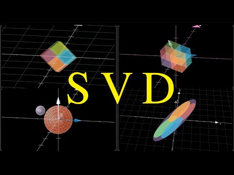
- In this video titled, “SVD Visualized and Explained”, you will learn how matrix rank captures information content, forming the mathematical basis of LoRA (Runtime: 16 mins)
- The video titled, “Eckart-Young: The Closest Rank k Matrix to A” by Prof Gilbert Strang from MIT, demonstrates why low-rank approximations are optimal, connecting directly to LoRA’s constrained updates (Runtime: 47 mins)

- In this video, Letitia Parcalabescu explains how to efficiently fine-tune Large Language Models. Shows how adapters are inserted into transformer architectures. (Runtime: 9 mins)

- This video titled, “SVD Gives the Best Low Rank Approximation” from Stanford”, provides a more theoretical recap of the LoRA fundamentals – great for reinforcing the key ideas (Runtime: 9 mins)

References
- Hu et al., LoRA: Low-Rank Adaptation of Large Language Models, arXiv:2106.09685
- Hugging Face PEFT documentation: https://huggingface.co/docs/peft
- Hugging Face blog: https://huggingface.co/blog/peft
- Microsoft Research GitHub: https://github.com/microsoft/LoRA
Related Articles
Author: Roy Gabriel, PhD Georgia Tech